Thursday, 31st July 2014

Chladni pattern is a n interesting example of Simple harmonic Motion. Today I devised a setup to produce these patterns using ExpEYES.

In Chladni patterns, points in an object undergo SHM with varying amplitudes. There will be some points where amplitude of SHM is zero, called nodes. If Small particles (sand / rangoli powder) are spread on the plate, they  collect at the nodes, ie along lines where the amplitude of SHM is small.

For the experimental Set-up I used a CD as Chladni plate. SQR1 is connected to  a small inductor (a coil of wire with no magnetic core) and produces a sinusoidal magnetic field. This is then placed close to a small magnet attached to the plate, and so produces a sinusoidal force on the magnet.

Two small magnets are placed on the edge of the plate. The inductor is placed so its centre is directly beneath the magnets and as close as possible to the plate without touching it.


Used python program to change frequency of SQR1.


Wednesday, 30th July 2014

Continued experimenting and exploring with coupled pendulums.

This link was of great help: Two coupled pendula

Today worked on python code for the experiment to generate waveforms, and now it is in its final form. Pushed the same to my GitHub repository.

Repeated the experiment in three different ways:

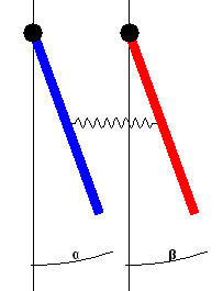
  • When both the pendulums oscillate in phase

coupledinphaseoscillating in fase


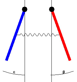
  • When  pendulums oscillate out of phase

coupledoutofphase

oscillating out of fase

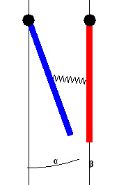
  • When one pendulum is at rest while the other is given oscillations

oscillating more complex

coupled pendula3

Now writing a simple GUI to access the code and experiment related information.

Tuesday, 29th July 2014

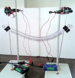
Oscillations of Coupled pendulum is an interesting phenomenon in Physics.

Two pendulum connected with a spring can be made to oscillate in different ways…

  • Both oscillating in phase
  • Both oscillating out of phase
  • One at rest and other oscillating

Today I could complete the experimental setup as well as the required python code.

Here is the experimental set-up….

cp1

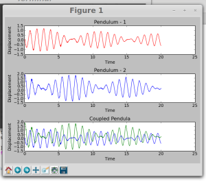
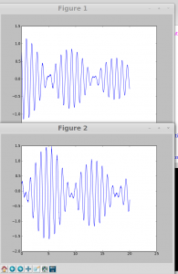
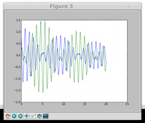
The waveforms generated using DC motors after amplification…

coupled pendula1 coupled pendula2 coupled pendula3

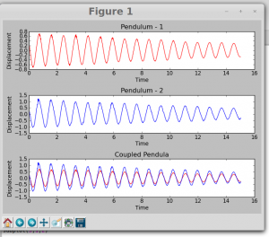
The waveforms show beats as theoretically expected….

The complete code is here…


Monday, 28th July 2014

Today I completed the program for resonance experiments ( tomorrow I will take some more trials with mic as detector) and continued to work on python codes for working with sensors – ultrasonic and photogate.

Started finalizing experiments with photo-gates. I may need another two days to complete everything, code and documentation of experiments with photo-sensors.

GSoC Weekly Report 10

( From Monday 21st July 2014 to Sunday, 27th July 2014)

I am happy with the work that I could do this week. Planning and basic set-up of almost all planned experiments for my GSoC project is complete. Gathered the required apparatus and set-ups are ready. Still some work on python programs for these experiments and documentation is to be done. In another week I will be able do complete the work. Then I can focus on polishing the code and finalizing everything.

Things we could do this week…..

  • Completed python program for using photo-gates for time measurements in various experiments. ( Some issues like timeout error are to be solved)
  • Started working on an interesting experiment of Helmholtz Resonator.
  • Wrote a python program to  digitize sound resulted from different resonators. With this program it is possible to change the frequency of source and when it matches with the natural frequency of resonator, a loud sound is produced. Tested the code with a bottle ( which resonates at about 200 Hz) and  a test tube (which resonates at about 450 Hz).
  • Python program ( srf3.py) to fetch data from srf module  and plot graphs needed some modifications to plot velocity and acceleration graphs. Now the basic program is complete and plots position, velocity and acceleration. Velocity is calculated using numerical differentiation and acceleration is calculated as the second derivative of position with numerical methods. Wrote following code for velocity and acceleration. Committed the entire program to GIT Repo.
  • In most of the mechanics experiments we are trying to plot multiple graphs ( position, velocity and acceleration or kinetic energy and potential energy etc.)  in one figure. In the figure the axis labels of two graphs are overlapping. These labels should have some spacing between them. Studied different functions available in python. I found tight-layout() function from matplotlib to be very easy and useful. Sometimes it can happen that axis labels or titles (or sometimes even ticklabels) go outside the figure area, and are thus clipped. tight_layout() can prevent this and also adjust spacing between subplots to minimize the overlaps.
  • The experiments of resonator and resonance tube are generally performed with tuning forks. Since tuning fork produces very low intensity sound, it is not clearly audible and the frequency is fixed. therefore the length of the resonance pipe must be changed to adjust with the frequency of tuning fork. We used a speaker connected to SQR1 of ExpEYES. frequency of SQR1 can be varied till we get sound of resonance. a wide range of frequencies is available from ExpEYES therefore it is easy to do this experiment with various sizes of tubes and resonators. We used a mic to study the amplitude. Wrote a python program to change frequency of SQR1 and to plot the frequency v/s amplitude graph. The program for frequency response study of pizzo buzzer was already available. Just made few modifications required for this experiment. I did experimental trials with a measuring flask, plastic pipe, conical flask and a round bottom flask.  Resonant frequency is between 300Hz to 750 Hz which varies with length of tube and volume of resonator.

Difficulties faced and things TO DO next week….

  • I am working on smoothing the graphs using filtering techniques. Wrote a program using Savitzky-Golay filtering ( From this source). I could remove all the errors in the program but not getting the plots. Need to work on it.
  • Ultrasonic sensor giving time-out error when used with get-echo program with SQR2 and IN1. It is working fine with SQR1 and SEN. Need to solve this issue.
  • Need to write a separate GUI for time, Speed and acceleration measurements using Photo-gates.
  • Complete Coupled pendula experimental set-up and python program.
  • Continue working on documentation.


Saturday, 26th July 2014

Today I worked on  Resonance Experiments using speaker instead of tuning fork.

The experiments of resonator and resonance tube are generally performed with tuning forks. Since tuning fork produces very low intensity sound, it is not clearly audible and the frequency is fixed. therefore the length of the resonance pipe must be changed to adjust with the frequency of tuning fork.

We used a speaker connected to SQR1 of ExpEYES. frequency of SQR1 can be varied till we get sound of resonance. a wide range of frequencies is available from ExpEYES therefore it is easy to do this experiment with various sizes of tubes and resonators. We used a mic to study the amplitude.

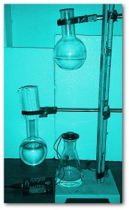
Here is the experimental set-up

resonance3 resonancesetupWrote a python program to change frequency of SQR1 and to plot the frequency v/s amplitude graph. The program for frequency response study of pizzo buzzer was already available. Just made few modifications required for this experiment.

I did experimental trials with a measuring flask, plastic pipe, conical flask and a round bottom flask.  Resonant frequency is between 300Hz to 750 Hz which varies with length of tube and volume of resonator.


Friday, 25th July 2014

In most of the mechanics experiments we are trying to plot multiple graphs ( position, velocity and acceleration or kinetic energy and potential energy etc.)  in one figure. In the figure the axis labels of two graphs are overlapping. These labels should have some spacing between them.

Today, while trying to solve this problem I got the information about tight-layout function from matplotlib (thanks to Google),

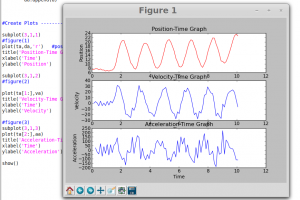
Here is the figure without tight-layout() function. The axis labels and titles are overlapped.

 subplots

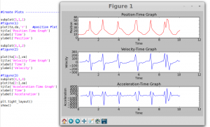
Sometimes it can happen that axis labels or titles (or sometimes even ticklabels) go outside the figure area, and are thus clipped. tight_layout() can prevent this and also adjust spacing between subplots to minimize the overlaps.

This figure is obtained using tight-layout() function…

subplotwithtightlayout

Today I have gathered required apparatus for performing various experiments like resonance and oscillations. Next two days I will set-up almost all planned experiments for my GSoC project.

Thursday, 24th July 2014

Python program ( srf3.py) to fetch data from srf module  and plot graphs needed some modifications to plot velocity and acceleration graphs. Today we could re-write the program to calculate velocity and acceleration. The program also plots position, velocity and acceleration.

Now I am working on smoothing the graphs using filtering techniques. Wrote a program using Savitzky-Golay filtering ( From this source). I could remove all the errors in the program but not getting the plots. Need to work on it.

Here is the screenshot of graphs obtained.

pva graph

Velocity is calculated using numerical differentiation and acceleration is calculated as the second derivative of position with numerical methods. Wrote following code for velocity and acceleration. Committed the entire program to GIT Repo.

——————————————————————————————————

va = []
aa = []
for i in range(0,len(da)-1):
# Calculate Velocity
v = (da[i+1]-da[i])/(ta[i+1]-ta[i])
va.append(v)
#aa= diff(va)

# Calculate Acceleration
if i < len(da)-2:
a = (da[i+2]-2*da[i+1]+da[i])/((ta[i+2]-ta[i+1])*(ta[i+1]-ta[i]))
aa.append(a)

—————————————————————————————————-

Wednesday, 23rd July 2014

Enjoyed setting-up sound resonance experiments. It really fun doing sound experiments with ExpEYES.

Polished the python code written yesterday. Now it is more flexible, user can digitize sound from any source and get the waveform on the screen. Using Xmgrace frequencies can be obtained.

Curve fitting function in the program is not giving correct results. It needs to be corrected.

Also with the new program we can vary the frequency of sound generated by the buzzer and one it matches with the natural frequency of resonator, a loud sound is generated. Used Helmholtz equation to relate frequency with volume.

Tried the code with different vessels, a bottle, a test tube a pipe and a round bottom flask (borrowed from chemistry lab.) Results are amazing.


Here is some useful information: (Source)

Some small whistles are Helmholtz oscillators. The air in the body of a guitar acts almost like a Helmholtz resonator. An ocarina is a slightly more complicated example, because for the higher notes it has several holes. Loudspeaker enclosures often use the Helmholtz resonance of the enclosure to boost the low frequency response. Here we analyse this oscillation, informally at first. Later, we derive the equation for the frequency of the Helmholtz resonance.


The vibration here is due to the ‘springiness’ of air: when you compress it, its pressure increases and it tends to expand back to its original volume. Consider a ‘lump’ of air at the neck of the bottle . The air jet can force this lump of air a little way down the neck, thereby compressing the air inside. That pressure now drives the ‘lump’ of air out but, when it gets to its original position, its momentum takes it on outside the body a small distance. This rarifies the air inside the body, which then sucks the ‘lump’ of air back in. It can thus vibrate like a mass on a spring . The jet of air from your lips is capable of deflecting alternately into the bottle and outside, and that provides the power to keep the oscillation going.
 

Tuesday, 22nd July 2014

Today I started working on an interesting experiment of Helmholtz Resonator.

A Helmholtz resonator is generally, a container of gas (usually air) with an open  neck or port. A volume of air in and near the open hole vibrates and produces audible sound with specific frequency. A common example is an empty bottle: the air inside vibrates when you blow across the top (It’s a fun experiment, because of the surprisingly low frequency and loud sound that results.)

I wrote a python program to  digitize sound resulted from different resonators. With this program it is possible to change the frequency of source and when it matches with the natural frequency of resonator, a loud sound is produced.

Tested the code with a bottle ( which resonates at about 200 Hz) and  a test tube (which resonates at about 450 Hz).

Tomorrow I will set up a complete experiment to study the phenomena of volume resonance.